 Earthquake Response Spectrum Analysis of 4 Story Shear Building
 Earthquake Response Spectrum Analysis of 4 Story Shear Building
[ Shear Building ]
[ Modal Analysis ]
[ Earthquake Response Spectrum ]
[ Modal Spectral Accelerations ]
[ Modal Displacements ]
[ Floor Displacements ]
[ Story Drifts ]
[ Inertia Forces ]
[ Shear Forces ]
[ Overturning Moments ]
[ Input and Output Files ]
In this example we compute the displacements, shear forces, story drifts, and over-turning moments in a 4 story shear structure subject to moderate earthquake loads.
Loads due to ground motions are represented by a scaled earthquake acceleration response spectrum.
Figure 1 is a schematic of the 4 story shear building, and its corresponding mass and stiffness matrices.
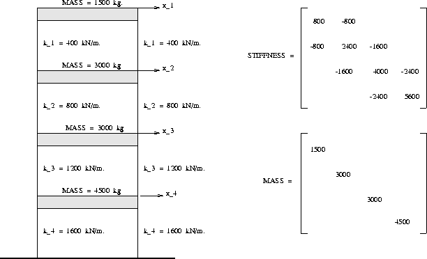
The vertical distance between floors is 3m (see computations on overturning moments below).
We assume that all of the building mass is lumped at the floor levels, that the floor beams are rigid, and that the columns are axially rigid. It follows from these assumptions that floor level displacements may be described by one degree-of-freedom alone, with only four degrees of freedom being needed to describe total displacements throughout the structure.
The mass and stiffness matrices are simply given by
    mass = ColumnUnits( 1500*[ 1, 0, 0, 0;
                               0, 2, 0, 0;
                               0, 0, 2, 0;
                               0, 0, 0, 3], [kg] );

    stiff = ColumnUnits( 800*[ 1, -1,  0,  0;
                              -1,  3, -2,  0;
                               0, -2,  5, -3;
                               0,  0, -3,  7], [kN/m] );
and generate the matrix ouput we are already familiar with.
The relevant block of ALADDIN code is:
   /* [c] : Calculate natural periods of vibration and mode shapes */

   no_eigen = 3;
   eigen       = Eigen( stiff, mass, [ no_eigen ] );
   eigenvalue  = Eigenvalue( eigen );
   eigenvector = Eigenvector ( eigen );

   period = ColumnUnits( Matrix( [ no_eigen,1 ] ), [ sec ] );
   for( ii = 1; ii <= no_eigen; ii = ii + 1 ) {
        period [ii][1] = 2*PI/sqrt(eigenvalue[ii][1]);
   }

   print "\n";
   for( ii = 1; ii <= no_eigen; ii = ii + 1 ) {
        print "Mode", ii, " : w^2 = ", eigenvalue[ii][1];
        print " T = ", period [ii][1], "\n";
   }

   PrintMatrix( eigenvector );
Ouput : Figure 2 shows the modal shapes and natural periods of vibration for the first three modes of the shear building
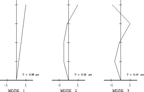
The textual output is as follows:
    *** SUBSPACE ITERATION CONVERGED IN 10 ITERATIONS

    Mode         1  : w^2 =      117.8 1/sec^2  T =     0.5789 sec
    Mode         2  : w^2 =      586.5 1/sec^2  T =     0.2595 sec
    Mode         3  : w^2 =       1125 1/sec^2  T =     0.1873 sec

    MATRIX : "eigenvector"

    row/col                  1            2            3
            units
       1            1.00000e+00  1.00000e+00 -9.00864e-01
       2            7.79103e-01 -9.96239e-02  1.00000e+00
       3            4.96553e-01 -5.39890e-01 -1.60784e-01
       4            2.35062e-01 -4.37612e-01 -7.05724e-01
    /*
     *  [a] : Setup Matrix for Piece-wise linear approximation to earthquake
     *        acceleration Spectra
     *
     *        Column 1 : Natural Period (sec)
     *        Column 2 : Spectral Acceleration (at 2% damping)
     */

    print "*** ACCELERATION SPECTRA FOR MODAL ANALYSIS \n";
    print "*** ======================================= \n";

    npoints = 18;
    spectra = Matrix( [ npoints , 2] );
    spectra = ColumnUnits( spectra, [sec],      [1]);
    spectra = ColumnUnits( spectra, [cm/sec^2], [2]);

    spectra [ 1][1] = 0.0 sec;  spectra [ 1][2] = 981.0*0.15 cm/sec/sec;
    spectra [ 2][1] = 0.1 sec;  spectra [ 2][2] = 981.0*0.18 cm/sec/sec;
    spectra [ 3][1] = 0.2 sec;  spectra [ 3][2] = 981.0*0.25 cm/sec/sec;
    spectra [ 4][1] = 0.3 sec;  spectra [ 4][2] = 981.0*0.38 cm/sec/sec;
    spectra [ 5][1] = 0.4 sec;  spectra [ 5][2] = 981.0*0.50 cm/sec/sec;
    spectra [ 6][1] = 0.5 sec;  spectra [ 6][2] = 981.0*0.50 cm/sec/sec;
    spectra [ 7][1] = 0.6 sec;  spectra [ 7][2] = 981.0*0.40 cm/sec/sec;
    spectra [ 8][1] = 0.8 sec;  spectra [ 8][2] = 981.0*0.32 cm/sec/sec;
    spectra [ 9][1] = 1.0 sec;  spectra [ 9][2] = 981.0*0.25 cm/sec/sec;
    spectra [10][1] = 1.2 sec;  spectra [10][2] = 981.0*0.19 cm/sec/sec;

    .... details of spectra removed .....

    spectra [18][1] = 3.4 sec;  spectra [18][2] = 981.0*0.02 cm/sec/sec;

    PrintMatrix( spectra );
defines a (18x2) matrix, spectra, for the acceleration response spectrum. The earthquake ground motions have a peak ground acceleration of 0.15 g.
The acceleration response spectra is represented as piecewise linear segments, whose end-points are defined by a (time, acceleration) coordinate.
Output : Figure 3 shows the lower- half of the earthquake acceleration response spectrum that we will use for the analysis.
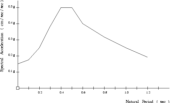
The textual counterpart to Figure 3 is:
    *** ACCELERATION SPECTRA FOR MODAL ANALYSIS
    *** =======================================

    MATRIX : "spectra"

    row/col                  1            2
            units          sec      m/sec^2
       1            0.00000e+00  1.47150e+00
       2            1.00000e-01  1.76580e+00

              ..... details removed ....

      17            3.20000e+00  1.96200e-01
      18            3.40000e+00  1.96200e-01
Now that we know the systems natural periods, the next step is to compute the spectral accelerations corresponding to each period.
The block of ALADDIN code:
    /* [d] : Find Spectral Accelerations at Modal Periods */

    SpectralAccn = ColumnUnits( Matrix( [ no_eigen,1 ] ), [ m/sec^2 ] );
    for( ii = 1; ii <= no_eigen; ii = ii + 1 ) {
        for( ij = 1; ij < npoints; ij = ij + 1 ) {
             period1 = spectra [  ij][1];
             period2 = spectra [ij+1][1];
             if(period [ii][1] >= period1 && period [ii][1] < period2 ) {
                dAccn   = spectra [ij+1][2] - spectra [ij][2];
                dPeriod = (period [ii][1] - period1)/(period2 - period1);
                SpectralAccn[ii][1] = spectra [ij][2] + dPeriod*dAccn;
             }
        }
    }

    PrintMatrix( SpectralAccn );
walks along the spectra array, and for each element in the matrix ``period'' (shown above), finds the spectral acceleration corresponding to natural period of the mode. Modal periods that fall between array values are estimated by linear interpolation.
Output : Figure 4 shows the acceleration response spectra with the modal periods and corresponding spectral accelerations superimposed.

The textual output from this computation is:
MATRIX : "SpectralAccn"

row/col                  1
        units
   1  m/sec^2   4.13122e+00
   2  m/sec^2   3.21070e+00
   3  m/sec^2   2.36550e+00
A quick comparison of the elements in ``period'' and ``spectra'' should reveal that these spectral accelerations match the computed natural periods.
The block of ALADDIN code:
    /* [e] : Generalised mass, stiffness, and loading matrices */

    eigenTrans = Trans (eigenvector);
    gmass      = eigenTrans*mass*eigenvector;
    gstiff     = eigenTrans*stiff*eigenvector;

    gload = eigenTrans*mass*[ 1; 1; 1; 1 ];

    PrintMatrix( gmass, gstiff, gload );

    /* [f] : Compute and print floor level displacements */

    Y = ColumnUnits( Matrix([no_eigen,no_eigen]), [ m ] );
    for( ii = 1; ii <= no_eigen; ii = ii + 1 ) {
         Y [ii][ii] = (gload[ii][1]/gmass[ii][ii]) *
                     (SpectralAccn[ii][1]/eigenvalue[ii][1]);
    }

    modaldispl = ColumnUnits ( eigenvector*Y, [cm]);
    PrintMatrix( Y , modaldispl );
computes modaldispl, a (4x3) matrix containing displacements in each mode. Ouput : Figure 5 shows the modal shapes and natural periods of vibration for the first three modes of the shear building
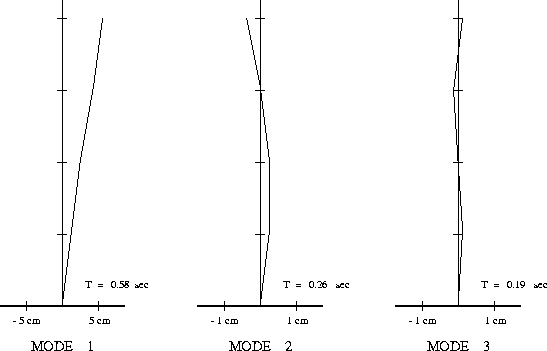
The textual output is:
    MATRIX : "gmass"

    row/col                  1            2            3
            units           kg           kg           kg
       1            4.30934e+03  2.84217e-13 -1.13687e-13
       2            1.13687e-13  3.26599e+03 -4.54747e-13
       3           -2.27374e-13 -2.27374e-13  6.53610e+03

    MATRIX : "gstiff"

    row/col                  1            2            3
            units          N/m          N/m          N/m
       1            5.07691e+05 -2.18279e-11  1.16415e-10
       2           -1.16415e-10  1.91539e+06 -1.16415e-10
       3            2.32831e-10 -2.32831e-10  7.35295e+06

    MATRIX : "gload"

    row/col                  1
            units
       1       kg   6.38475e+03
       2       kg  -2.38779e+03
       3       kg  -2.00941e+03

    MATRIX : "Y"

    row/col                  1            2            3
            units            m            m            m
       1            5.19545e-02  0.00000e+00  0.00000e+00
       2            0.00000e+00 -4.00257e-03  0.00000e+00
       3            0.00000e+00  0.00000e+00 -6.46441e-04

    MATRIX : "modaldispl"

    row/col                  1            2            3
            units           cm           cm           cm
       1            5.19545e+00 -4.00257e-01  5.82355e-02
       2            4.04779e+00  3.98752e-02 -6.46441e-02
       3            2.57982e+00  2.16095e-01  1.03938e-02
       4            1.22125e+00  1.75157e-01  4.56209e-02
Points to note:
    print "\n";
    print "Maximum Possible Floor Displacements (absolute values) \n";
    print "====================================================== \n\n";
    print "     Floor          Mode         Modes         Modes\n";
    print "        No             1         1 & 2    1, 2 and 3\n";

    for( ii = 1; ii <= 4; ii = ii + 1 ) {
        print (5-ii);
        for( ij = 1; ij <= no_eigen; ij = ij + 1 ) {
             sum = 0.0 cm;
             for( ik = 1; ik <= ij; ik = ik + 1 ) {
                  sum = sum + abs( modaldispl [ii][ik] );
             }
             print sum (cm);
        }
        print "\n";
    }
Ouput : Results are presented for mode 1 alone,
modes 1 and 2, and modes 1 to 3.
    Maximum Possible Floor Displacements (absolute values)
    ======================================================

         Floor          Mode         Modes         Modes
            No             1         1 & 2    1, 2 and 3
             4      5.195 cm      5.596 cm      5.654 cm
             3      4.048 cm      4.088 cm      4.152 cm
             2       2.58 cm      2.796 cm      2.806 cm
             1      1.221 cm      1.396 cm      1.442 cm
Clearly, mode 1 makes the greatest contribution to overall floor displacements.
In the block of ALADDIN code:
    /* [g] : Compute and print story drifts */

    print "\n";
    print "Maximum Likely Story Drifts (using SRSS) \n";
    print "======================================== \n\n";
    print "     Story          Mode         Modes         Modes\n";
    print "        No             1         1 & 2    1, 2 and 3\n";

    for( ii = 1; ii <= 4; ii = ii + 1 ) {
        print (5-ii);
        for( ij = 1; ij <= no_eigen; ij = ij + 1 ) {
             sum = 0.0 cm^2;
             for( ik = 1; ik <= ij; ik = ik + 1 ) {
                  if (ii == 4) then {
                      sum = sum + modaldispl[4][ik]^2;
                  } else {
                      sum = sum + (modaldispl [ii][ik] - modaldispl [ii+1][ik])^2;
                  }
             }
             print sqrt(sum) (cm);
        }
        print "\n";
    }
we compute the maximum likely story drift at each floor using mode 1 alone, modes 1 and 2, and modes 1 to 3. Maximum likely story drift is taken as the square root of the sum of story drifts squared.
Ouput : The output
    Maximum Likely Story Drifts (using SRSS)
    ========================================

         Story          Mode         Modes         Modes
            No             1         1 & 2    1, 2 and 3
             4      1.148 cm      1.229 cm      1.235 cm
             3      1.468 cm      1.479 cm       1.48 cm
             2      1.359 cm      1.359 cm       1.36 cm
             1      1.221 cm      1.234 cm      1.235 cm
shows that most of the story drifts occur in modes 1 and 2.
    /* [h] : Compute and print equivalent d.o.f. forces in each mode */

    print "\n";
    print "Inertia Forces for each mode \n";
    print "============================ \n\n";

    inertia_forces = stiff*modaldispl;
    PrintMatrix( inertia_forces );
Ouput : Figure 6 shows the distribution of inertia forces
in each of the first three modes of vibration.
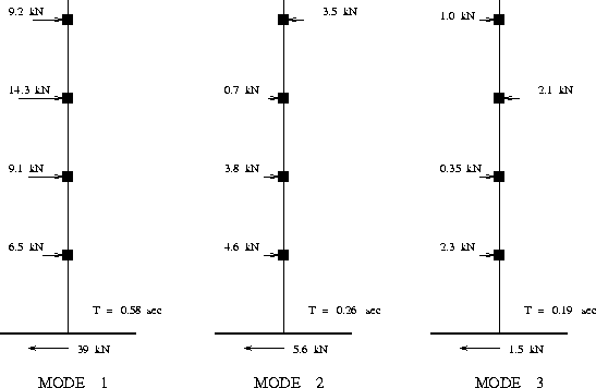
The textual output is:
    Inertia Forces for each mode
    ============================

    MATRIX : "inertia_forces"

    row/col                  1            2            3
            units            N            N            N
       1            9.18127e+03 -3.52106e+03  9.83037e+02
       2            1.43063e+04  7.01546e+02 -2.18364e+03
       3            9.11798e+03  3.80201e+03  3.55155e+02
       4            6.47450e+03  4.62254e+03  2.30532e+03
In the block of ALADDIN code:
    /* [i] : Compute and print base shear force */

    print "\n";
    print "Shear Forces (at base of the structure) \n";
    print "======================================= \n\n";

    base_shear_forces = [1,1,1,1] * inertia_forces;
    PrintMatrix( base_shear_forces );

    shear1 = 0.0 N^2; shear2 = 0.0 N;
    for ( ii = 1; ii <= no_eigen; ii = ii + 1 ) {
         shear1 = shear1 + base_shear_forces[ 1 ][ ii ]^2;
         shear2 = shear2 + abs( base_shear_forces[ 1 ][ ii ] );
    }

    print "\n";
    print "Base Shear Force : Maximum Likely   = ", sqrt(shear1) ,"\n";
    print "                 : Maximum Possible = ", shear2       ,"\n";
we compute the base shear force for each mode by simply premultiplying the "inertia forces" by a sumation vector [1,1,1,1].
Ouput : The maximum likely and maximum possible base shear force is given by the square root of the sum of shear forces squared, and sum of absolutio shear forces, respectively.
    Shear Forces (at base of the structure)
    =======================================

    MATRIX : "base_shear_forces"

    row/col                  1            2            3
            units            N            N            N
        1            3.90800e+04  5.60504e+03  1.45987e+03

    Base Shear Force : Maximum Likely   =  3.951e+04 N
                     : Maximum Possible =  4.614e+04 N
Here we see that most of the base shear force is due to inertia forces in modes 1 and 2.
Input : For each mode, the overturning moment is given by the sum of inertia forces times the vertical distance from the base.
    /* [j] : Compute and print overturning moments */

    print "\n";
    print "Overturning Moments (at base of the structure) \n";
    print "============================================== \n\n";

    floor_heights            = [12 m, 9 m, 6 m, 3 m];
    base_overturning_moments = floor_heights * inertia_forces;
    PrintMatrix( base_overturning_moments );

    mom1 = 0.0 (N*m)^2; mom2 = 0.0 N*m;
    for ( ii = 1; ii <= no_eigen; ii = ii + 1 ) {
          mom1 = mom1 + base_overturning_moments[ 1 ][ ii ]^2;
          mom2 = mom2 + abs( base_overturning_moments[ 1 ][ ii ] );
    }
Here we assume that the floors are spaced 3 m apart.
Ouput : The generated output:
    Overturning Moments (at base of the structure)
    ==============================================

    MATRIX : "base_overturning_moments"

    row/col                  1            2            3
            units          N.m          N.m          N.m
       1            3.13063e+05  7.40882e+02  1.19055e+03

    Overturning Moments : Maximum Likely   =  3.131e+05 N.m
                        : Maximum Possible =   3.15e+05 N.m
shows the overturning moments for modes 1 through 3, and the maximum likely and maximum possible overturning momemts.
Once again, we use the square root of the sum of the squares for likely overturning moments, and the sum of absolute values for maximum possible overturning moments.