[ Problem Statement ] [ Finite Element Mesh ] [ Displacement Calculation ] [ Displaced Cantilever ] [ Element-Level Forces ] [ Input/Output Files ]
You will need Aladdin 3.0 to run this problem.
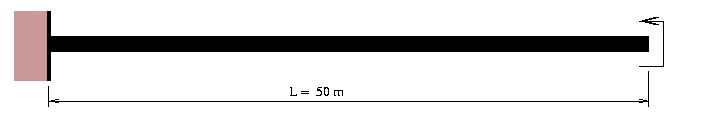
In this example, we use the two-dimensional geometrically exact rod model developed by Simo and Vu Quoc [1,2] to compute the displacements of a long slender cantilever beam subject to an end moment. See Figure 1.
Theoretical considerations indicate that when the end moment is:
M = 2*PI*(EI/L)
the rod will roll into a complete circle. We assume that Izz = 100 m^4 and the cross-section area A = 0.0001 m^2. The material properties are Young's modulus E = 10000 Pa, Poisson's ration = 0.25.
Because the pipe cross section has axes of symmetry on both the horizontal and vertical axes, we need only model 1/4 of the pipe cross section.
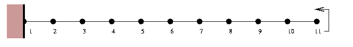
Figure 2 shows the finite element mesh for the cantilever rod. The block of code:
/* Generate line of nodes */

   for(node = 1; node <= 11; node = node + 1) {
       AddNode(node, [ (node-1)*5 m,  0 m ] );
   }

/* Attach beam elements to nodes */

   for(elmtno = 1; elmtno <= 10; elmtno = elmtno + 1) {
       AddElmt( elmtno, [ elmtno, elmtno + 1 ], "rodproperties");
   }
generates a line of 11 nodes and 10 beam finite element:
    =========================   =========================
    Node      x (m)     y (m)   Element    node 1  node 2
    =========================   =========================
       1        0.0       0.0         1         1       2
       2        5.0       0.0         2         2       3

       ...........

      10       45.0       0.0        10        10      11
      11       50.0       0.0   =========================
    =========================
Section and Material Properties
The block of code:
   ElementAttr("rodproperties") { type     = "GEXACT_2D";
                                  section  = "rodsection";
                                  material = "rodmaterial";
                                }

   SectionAttr("rodsection") { Izz       =    100 m^4;
                               area      = 0.0001 m^2;
                             }

   MaterialAttr("rodmaterial") { poisson = 0.25;
                                 E       = 10000 Pa;
                               }
defines the material and section properties for the "rod" finite element.
Boundary Conditions
We assume that the cantilever is fully fixed at its base:
   nodeno = 1;
   FixNode( nodeno, [ 1, 1, 1 ]);
After the boundary conditions have been applied, the finite element model has 30 degrees of freedom.
External Loads
The cantilever is subject to an end moment
NodeLoad( 11, [ 0.0 N, 0.0 N, 2*PI*20000 N*m ]);
that will roll it into a circle. The initial configuration is as follows:
    *** ======================================
    *** Initial Configuration
    *** L2norm(unbalance force) =  1.257e+05
    *** Relative error : err = 1.0
    *** ======================================
    Node :          1  x =          0 m  y =          0 m
    Node :          2  x =          5 m  y =          0 m
    Node :          3  x =         10 m  y =          0 m
    Node :          4  x =         15 m  y =          0 m
    Node :          5  x =         20 m  y =          0 m
    Node :          6  x =         25 m  y =          0 m
    Node :          7  x =         30 m  y =          0 m
    Node :          8  x =         35 m  y =          0 m
    Node :          9  x =         40 m  y =          0 m
    Node :         10  x =         45 m  y =          0 m
    Node :         11  x =         50 m  y =          0 m
The abbreviated block of statements:
   x = L2Norm(eload);
   tol = 0.0000001;
   err = 1 + tol;
   while( err > tol ) {

      i = i + 1;

      /* Save displacement to database      */

      ElmtStateDet( displ );
      UpdateResponse();

      /* Compute tangent stiffness          */

      stiff = Stiff();

      /* Compute internal load matrix       */

      Fs = InternalLoad( displ );

      /* Compute vector of unbalance forces */

      Unbalance = eload - Fs;

      /* Compute increment in displcement   */

      d_displ = Solve(stiff, Unbalance) ;

      /* Update displacement vector */

      displ = displ + d_displ;

      /* Compute relative error in unbalance force */

      y = L2Norm(Unbalance);
      err = y/x;

      /* Compute and print coordinates at ith iteration */

      ..... details removed .....

   }
shows the essential details of the iterative procedure for the displacement calculation. Five iterations are needed to achieve the required convergence in displacments and unbalance force. The change in unbalance force versus iteration no is as follows:
    Iteration No    L2Norm (unbalance forces)    Relative Error (y/x)
    ------------    -------------------------    --------------------
               0                    1.257e+05                     1.0
               1                         39.8               0.0003168
               2                        236.7                0.001884
               3                        15.59               0.0001241
               4                       0.3496               2.782e-06
               5                     0.004895               3.896e-08
    ------------    -------------------------    --------------------
The nodal displacements are as follows:
    ============================================================
     Node                           Displacement
       No            displ-x           displ-y             rot-z
    ============================================================
    units                m                 m               rad
       1         0.00000e+00       0.00000e+00       0.00000e+00
       2        -4.21012e-01       1.48780e+00       6.28317e-01
       3        -2.59103e+00       5.38290e+00       1.25663e+00
       4        -7.59101e+00       1.01975e+01       1.88495e+00
       5        -1.54209e+01       1.40927e+01       2.51327e+00
       6        -2.49999e+01       1.55805e+01       3.14158e+00
       7        -3.45789e+01       1.40928e+01       3.76990e+00
       8        -4.24089e+01       1.01977e+01       4.39822e+00
       9        -4.74090e+01       5.38304e+00       5.02653e+00
      10        -4.95791e+01       1.48787e+00       5.65485e+00
      11        -5.00001e+01      -1.67447e-05       6.28317e+00
    ============================================================
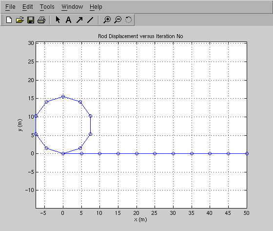
Coordinates of the displaced rod are obtained by adding the nodal displacements to the nodal coordinates of the unloaded system. This gives:`
Coordinates of Displaced Rod
============================
         1          0 m          0 m
         2      4.579 m      1.488 m
         3      7.409 m      5.383 m
         4      7.409 m       10.2 m
         5      4.579 m      14.09 m
         6   8.56e-05 m      15.58 m
         7     -4.579 m      14.09 m
         8     -7.409 m       10.2 m
         9     -7.409 m      5.383 m
        10     -4.579 m      1.488 m
        11 -0.0001491 m -1.674e-05 m
See Figure 3.
The aladdin statement:
PrintStress(displ);
computes and prints the element-level forces in the displaced cantilever. A summary of the output is as follows:
MEMBER FORCES
------------------------------------------------------------------------------

Elmt No   1 :
Coords : (x1, y1) = (     0.000 m ,      0.000 m)
       : (x2, y2) = (     5.000 m ,      0.000 m)

 Fx1 =   2.52081e-08 N  Fy1 =  -1.06192e-07 N  Mz1 =  -1.25664e+05 N.m
 Fx2 =  -2.52081e-08 N  Fy2 =   1.06192e-07 N  Mz2 =   1.25664e+05 N.m

 .... lines of output removed ....

Elmt No   9 :
Coords : (x1, y1) = (    40.000 m ,      0.000 m)
       : (x2, y2) = (    45.000 m ,      0.000 m)

 Fx1 =  -2.45165e-07 N  Fy1 =   1.41412e-07 N  Mz1 =  -1.25664e+05 N.m
 Fx2 =   2.45165e-07 N  Fy2 =  -1.41412e-07 N  Mz2 =   1.25664e+05 N.m


Elmt No  10 :
Coords : (x1, y1) = (    45.000 m ,      0.000 m)
       : (x2, y2) = (    50.000 m ,      0.000 m)

 Fx1 =  -1.16294e-07 N  Fy1 =  -1.25033e-08 N  Mz1 =  -1.25664e+05 N.m
 Fx2 =   1.16294e-07 N  Fy2 =   1.25033e-08 N  Mz2 =   1.25664e+05 N.m
------------------------------------------------------------------------------
Points to note:
Developed in 2000 by Mark Austin,
Copyright © 2000, Mark Austin, University of Maryland.